
Recommended

Predict Forex candlestick patterns using Keras.

Check accuracy of candlestick patterns on FOREX dataset
The problem:
Check if it is possible to predict forex price movements only based on candlestick data. We will use 1h time-frame data set of EUR/USD during ~2014-2019 year. We will take only 3 last candles and based on that make a prediction of the next candle.
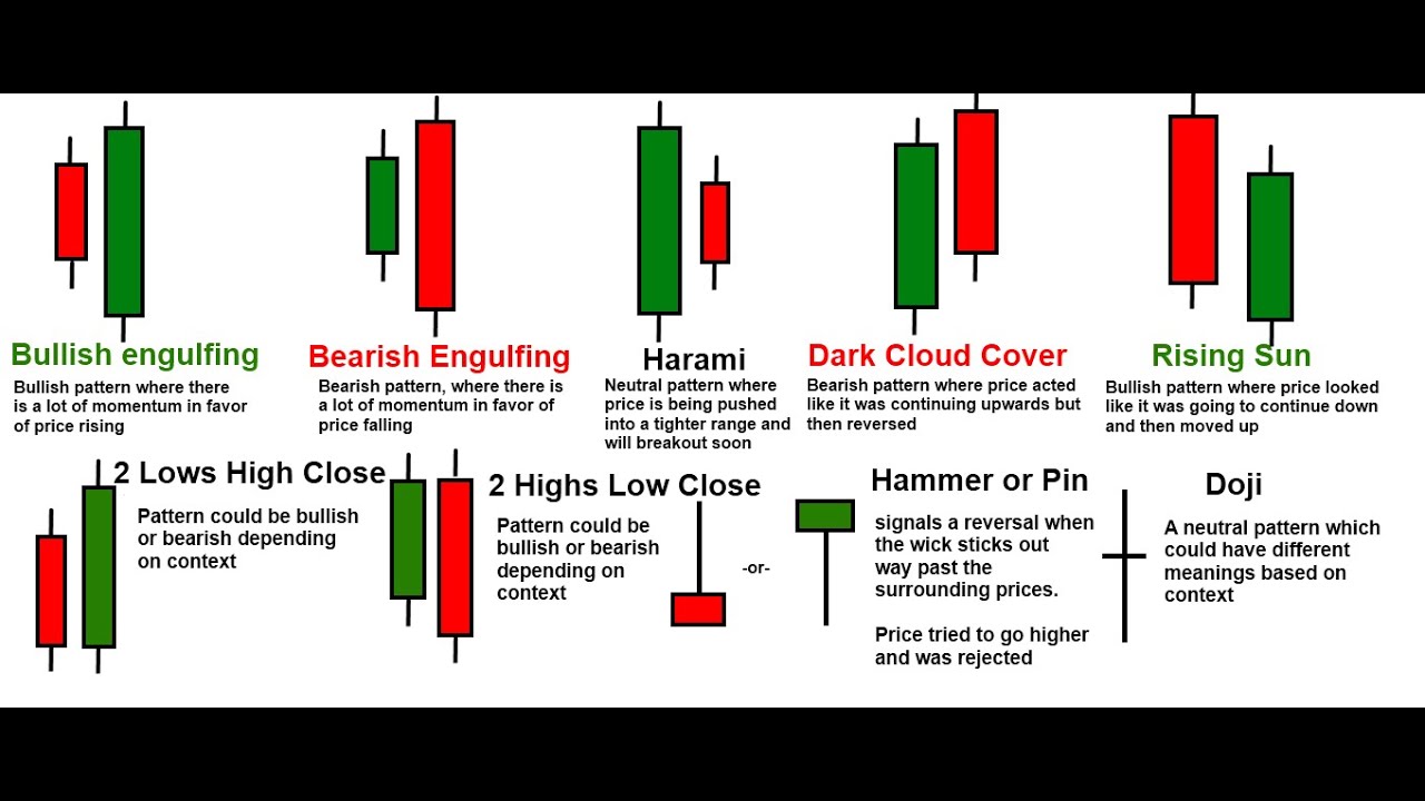
The example of candlestick patterns that we will try to predict or prove that those kind of patterns exists and work:
Before we even start, we need to download all the required libraries to perform the task.
import matplotlib
import numpy as np
import pandas as pd
import itertools
import sklearn
import keras
import time
import shap


from keras.models import Sequential
from keras.layers import Dense, Dropout, CuDNNLSTM, Conv1D
from matplotlib import pyplot as plt
from sklearn import preprocessing

from sklearn.model_selection import train_test_split
import matplotlib.pyplot as plt
import matplotlib.ticker as mticker
from mpl_finance import candlestick_ohlc


print('Numpy version: ' + np.__version__)
print('Pandas version: ' + pd.__version__)
print('Matplotlib version: ' + matplotlib.__version__)
print('Sklearn version: ' + sklearn.__version__)
print('Keras version: ' + keras.__version__)
Numpy version: 1.16.4
Pandas version: 0.24.2
Matplotlib version: 3.1.0
Sklearn version: 0.21.2
Keras version: 2.2.4
Class object to measure time
class MeasureTime:
    def __init__(self):
        self.start = time.time()
    def kill(self):
        print ('Time elapsed: ' + time.strftime("%H:%M:%S", time.gmtime(time.time()-self.start)))
        del self
Notebook_timer = MeasureTime()
Notebook_timer.kill()
Time elapsed: 00:00:01
1.1 - Import the dataset
We will download our historical dataset from ducascopy website in form of CSV file. https://www.dukascopy.com/trading-tools/widgets/quotes/historical_data_feed
my_dataset = pd.read_csv('EURUSD_1H_2014_2019.csv')
Check the imported data
del my_dataset['Gmt time']
del my_dataset['Volume']
my_dataset.head(5)
| Open | High | Low | Close | |
|---|---|---|---|---|
| 0 | 1.31950 | 1.31956 | 1.31942 | 1.31954 |
| 1 | 1.31954 | 1.31954 | 1.31954 | 1.31954 |
| 2 | 1.31954 | 1.31954 | 1.31954 | 1.31954 |
| 3 | 1.31954 | 1.31954 | 1.31954 | 1.31954 |
| 4 | 1.31954 | 1.31954 | 1.31954 | 1.31954 |
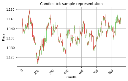
Let’s visualize it on the actual OHLC candlestick chart.
In order to do that we need to make our own function that will plot the OHLC data on the chart. We will use matplotlib library with finnance extension called mpl_finance. But before that, we need prepare out dataset to be in 3 dimensional arre with format (Timestep, Items, Features)
Timestep = List of candles seqeuence
Items = Candlestick
Features = High, Low, Open, Close parametes
Function to plot OHLC candlestick data in to chart
def graph_data_ohlc(dataset):
    fig = plt.figure()
    ax1 = plt.subplot2grid((1,1), (0,0))
    closep=dataset[:,[3]]
    highp=dataset[:,[1]]
    lowp=dataset[:,[2]]
    openp=dataset[:,[0]]
    date=range(len(closep))

    x = 0
    y = len(date)
    ohlc = []
    while x < y:
        append_me = date[x], openp[x], highp[x], lowp[x], closep[x]
        ohlc.append(append_me)
        x+=1
    candlestick_ohlc(ax1, ohlc, width=0.4, colorup='#77d879', colordown='#db3f3f')
    for label in ax1.xaxis.get_ticklabels():
        label.set_rotation(45)
    ax1.xaxis.set_major_locator(mticker.MaxNLocator(10))
    ax1.grid(True)
    plt.xlabel('Candle')
    plt.ylabel('Price')
    plt.title('Candlestick sample representation')

    plt.subplots_adjust(left=0.09, bottom=0.20, right=0.94, top=0.90, wspace=0.2, hspace=0)
    plt.show()
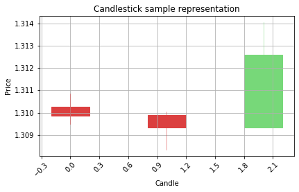
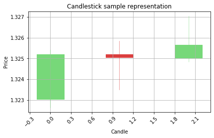
Visualize 1000 candlesticks on the OHLC chart in one time
graph_data_ohlc(my_dataset.tail(1000).values)
1.2 - Converting data to time series format
In order for our machine to learrn from our data, we need to change the format of the data we provide for learning. Most of the human traders do not watch the price but instead, they watch how candlesticks form on the chart and for patterns there. We will look for patterns based on the last 3 candles. To do so, we need to change the format of our dataset to 3 dimensional array (Timestep, Items, Features) .
Custom generator function to create 3d arrays of candles sequence
def my_generator(data,lookback):
    final_output = []
    counter = 0
    first_row = 0
    arr = np.empty((1,lookback,4), int)
    for a in range(len(data)-lookback):
        temp_list = []
        for candle in data[first_row:first_row+lookback]:
            temp_list.append(candle)
        temp_list2 = np.asarray(temp_list)
        templist3 = [temp_list2]
        templist4 = np.asarray(templist3)
        arr = np.append(arr, templist4, axis=0)
        first_row=first_row+1
    return arr
cell_timer = MeasureTime()
three_dim_sequence = np.asarray(my_generator(my_dataset.values[1:],3))
cell_timer.kill()
Let’s check the shape of our 3 dimension array, we got: 37557 sequences of 3 candles, each candle has 4 parameters.
three_dim_sequence.shape
(37557, 3, 4)
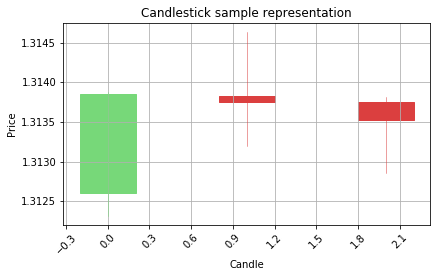
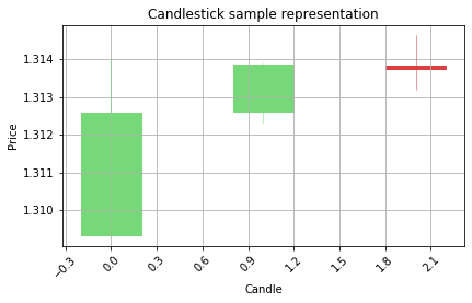
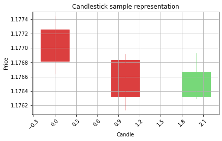
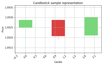
OK, now it is time to see how our sequence of 3 candlesticks looks like on the actual chart
Visualize the step by step sequency of price movements on the OHLC chart
counter=0
for candle in three_dim_sequence[1000:1005]:
    counter=counter+1
    print('Step ' + str(counter))
    graph_data_ohlc(candle)
Step 1

Step 2

Step 3

Step 4

Step 5
1.3 - Feature engineering
Now it is time to convert the price data in to actual candlestick parameters. Each candle has 4 parameters:
- Size of the body measured by pips
- Size of the upper wicks measured by pips
- Size of the lower wicks measured by pips
- Type of the candle (Bullish or Bearish)(Green or Red)(0 or 1)
pip = diffrence between 2 prices multiplied by 10000
(The whole process of enriching the raw dataset is called ‘feature engineering’)
Function to convert OHLC data in to candlestick parameters data
def ohlc_to_candlestick(conversion_array):
    candlestick_data = [0,0,0,0]

    if conversion_array[3]>conversion_array[0]:
        candle_type=1
        wicks_up=conversion_array[1]-conversion_array[3]
        wicks_down=conversion_array[2]-conversion_array[0]
        body_size=conversion_array[3]-conversion_array[0]

    else:
        candle_type=0
        wicks_up=conversion_array[1]-conversion_array[0]
        wicks_down=conversion_array[2]-conversion_array[3]
        body_size=conversion_array[1]-conversion_array[3]


    if wicks_up < 0:wicks_up=wicks_up*(-1)
    if wicks_down < 0:wicks_down=wicks_down*(-1)
    if body_size < 0:body_size=body_size*(-1)
    candlestick_data[0]=candle_type
    candlestick_data[1]=round(round(wicks_up,5)*10000,2)
    candlestick_data[2]=round(round(wicks_down,5)*10000,2)
    candlestick_data[3]=round(round(body_size,5)*10000,2)

    return candlestick_data
Lets extract data of only one candle from our dataset of sequences
cell_timer = MeasureTime()
one_candle_data_ohlc=three_dim_sequence[1000:1010][5][1]
cell_timer.kill()
one_candle_data_ohlc
array([1.31375, 1.31381, 1.31286, 1.31353])
Convert it to candlestick parameters
one_candle_data_ohlc_candle=ohlc_to_candlestick(one_candle_data_ohlc)
one_candle_data_ohlc_candle
[0, 0.6, 6.7, 2.8]
Apply this function in to generator function to get sequences with candlestick data instead of OHLC data
def my_generator_candle(data,lookback):
    first_row = 0
    arr = np.empty((1,lookback,4), int)
    for a in range(len(data)-lookback):
        temp_list = []
        for candle in data[first_row:first_row+lookback]:
            converted_data = ohlc_to_candlestick(candle)
            temp_list.append(converted_data)
        temp_list2 = np.asarray(temp_list)
        templist3 = [temp_list2]
        templist4 = np.asarray(templist3)
        arr = np.append(arr, templist4, axis=0)
        first_row=first_row+1
    return arr
Get the get the data in form of sequences made from last 3 candles
three_dim_sequence_candle=my_generator_candle(my_dataset.values[1:],3)
Check if conversion applied correctly
three_dim_sequence_candle[5000:5005]
array([[[ 0. ,  3.2,  8.6, 10. ],
        [ 1. ,  2.2,  8.2, 11. ],
        [ 0. ,  2.5,  9.1,  2.7]],

       [[ 1. ,  2.2,  8.2, 11. ],
        [ 0. ,  2.5,  9.1,  2.7],
        [ 1. ,  6.2,  3.2,  5.3]],

       [[ 0. ,  2.5,  9.1,  2.7],
        [ 1. ,  6.2,  3.2,  5.3],
        [ 0. ,  0.6,  5.4, 16.2]],

       [[ 1. ,  6.2,  3.2,  5.3],
        [ 0. ,  0.6,  5.4, 16.2],
        [ 0. ,  3.4,  6. ,  7.4]],

       [[ 0. ,  0.6,  5.4, 16.2],
        [ 0. ,  3.4,  6. ,  7.4],
        [ 1. ,  4.8,  8.8,  0.1]]])
Generate forecasting data
Now we have our candlestick values in the correct format for machine to read it and interpret it so, it is time to generete our prediction/forecasting data.
The idea was to predict the next candle type (bullish or bearish) by looking on for the last 3 candles. We got our sequences of 3 candles and now we need to generate another array with one candle information, which we will be forecasting.
Update of the generator to return one more array with 1 or 0 (Bullish or Bearish)
def my_generator_candle_X_Y(data,lookback,MinMax = False):
    if MinMax==True:scaler = preprocessing.MinMaxScaler()
    first_row = 0
    arr = np.empty((0,lookback,4))
    arr3 = np.empty((0,lookback,4))
    Y_list = []
    for a in range(len(data)-lookback):
        temp_list = []
        temp_list_raw = []
        for candle in data[first_row:first_row+lookback]:
            converted_data = ohlc_to_candlestick(candle)
            temp_list.append(converted_data)
            temp_list_raw.append(candle)
        temp_list3 = [np.asarray(temp_list)]
        templist4 = np.asarray(temp_list3)

        if MinMax==True:
            templist99 = scaler.fit_transform(templist4[0])
            arr = np.append(arr, [templist99], axis=0)
        else:
            arr = np.append(arr, templist4, axis=0)

        temp_list7 = [np.asarray(temp_list_raw)]
        templist8 = np.asarray(temp_list7)
        arr3 = np.append(arr3, templist8, axis=0)

        converted_data_prediction = ohlc_to_candlestick(data[first_row+lookback])
        Prediction = converted_data_prediction[0]
        Y_list.append(Prediction)

        first_row=first_row+1

    arr2 = np.asarray(Y_list)

    return arr,arr2,arr3
We will call the function and receive 2 datasets:
X = Input dataset on which our neural network will make predictions
Y = Prediction dataset (results of the correct predictions)
cell_timer = MeasureTime()
X,Y, X_raw = my_generator_candle_X_Y(my_dataset.values,3,MinMax=False)
cell_timer.kill()
Exploring the genereted dataset:
print('Shape of X ' + str(X.shape))
print('Shape of Y ' + str(Y.shape))
print('Shape of X raw ohlc ' + str(X_raw.shape))
Shape of X (37557, 3, 4)
Shape of Y (37557,)
Shape of X raw ohlc (37557, 3, 4)
X[653]
array([[ 1. ,  4.5,  0.3, 15.8],
       [ 1. ,  2.6,  1. ,  9. ],
       [ 0. ,  6.3,  7.2, 13.8]])
Y[653]
1
X_raw[653]
array([[1.35109, 1.35312, 1.35106, 1.35267],
       [1.35267, 1.35383, 1.35257, 1.35357],
       [1.3536 , 1.35423, 1.35213, 1.35285]])
How many bullish and bearish predictions?
unique, counts = np.unique(Y, return_counts=True)
predictions_type = dict(zip(unique, counts))
print('Bull: ' + str((predictions_type[1])) + ' percent: ' + str(round((predictions_type[1]*100)/len(Y),2)) + '%')
print('Bear: ' + str((predictions_type[0])) + ' percent: ' + str(round((predictions_type[0]*100)/len(Y),2)) + '%')
print('Total: ' + str(len(Y)))
Bull: 18622 percent: 49.58%
Bear: 18935 percent: 50.42%
Total: 37557
Now we know that our data for predictions is distributed equally.
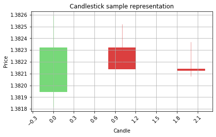
Visualize the candle sequence:
for a in range(5):
    b=a+1000
    if Y[b] == 1:print('Correct prediction would be Bullish ---^')
    if Y[b] == 0:print('Correct prediction would be Bearish ---v')
    graph_data_ohlc(X_raw[b])
Correct prediction would be Bullish ---^
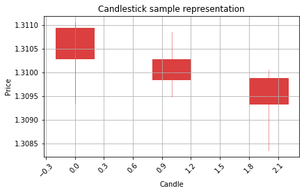
Correct prediction would be Bullish ---^
Correct prediction would be Bearish ---v

Correct prediction would be Bearish ---v
Correct prediction would be Bullish ---^

1.4 - Build Deep Learning model
For all sequence dataset the best model are RNN - Recurrent neural network. For our case we will build the LSTM network ( Long-Term Short-Term)
The basics, for all the training and prediction will be responsible the tensorflow library, with high level API called KERAS.
Defining the model
from keras import layers
from keras.optimizers import RMSprop


model = Sequential()
model.add(layers.CuDNNLSTM(units = 12,return_sequences=True, input_shape = (None, X.shape[-1])))
model.add(layers.CuDNNLSTM(units = 24))
model.add(layers.Dense(units = 1,activation='sigmoid'))

model.compile(optimizer='rmsprop', loss='binary_crossentropy', metrics=['acc'])
The model is build from 2 LSTM layers with 12,24 units(so called neurons). More layers and more units we add, more details our model will catch. But there is also a risk, if we add more “space” for model to learn, the model can quickly overfit the trainig data.
Overfiting - Model learned from the data set patterns that describe only the traning dataset. There is no big overview common pattern but instead a lot of small patterns that only apply to traning dataset. In machine learning field there is always a conflict between undertraining and overfitting the model.
Definition of the compiled model
model.summary()
Model: "sequential_7"
_________________________________________________________________
Layer (type)                 Output Shape              Param #
=================================================================
cu_dnnlstm_15 (CuDNNLSTM)    (None, None, 12)          864
_________________________________________________________________
cu_dnnlstm_16 (CuDNNLSTM)    (None, 24)                3648
_________________________________________________________________
dense_6 (Dense)              (None, 1)                 25
=================================================================
Total params: 4,537
Trainable params: 4,537
Non-trainable params: 0
_________________________________________________________________
In order train the deep learning model we need to split our data for 3 parts:
- Traning dataset
- Validation dataset
- Test dataset
cell_timer = MeasureTime()
X_train, X_val_and_test, Y_train, Y_val_and_test = train_test_split(X, Y, test_size=0.5)
X_val, X_test, Y_val, Y_test = train_test_split(X_val_and_test, Y_val_and_test, test_size=0.5)

X_train_raw, X_val_and_test_raw= train_test_split(X_raw, test_size=0.5)
X_val_raw, X_test_raw = train_test_split(X_val_and_test_raw, test_size=0.5)
cell_timer.kill()
print('Training data: ' + 'X Input shape: ' + str(X_train.shape) + ', ' + 'Y Output shape: ' + str(Y_train.shape) + ', ' + 'datetime shape: ' + str(Y_train.shape))
print('Validation data: ' + 'X Input shape: ' + str(X_val.shape) + ', ' + 'Y Output shape: ' + str(Y_val.shape) + ', ' + 'datetime shape: ' + str(Y_val.shape))
print('Test data: ' + 'X Input shape: ' + str(X_test.shape) + ', ' + 'Y Output shape: ' + str(Y_test.shape) + ', ' + 'datetime shape: ' + str(Y_test.shape))
Training data: X Input shape: (18778, 3, 4), Y Output shape: (18778,), datetime shape: (18778,)
Validation data: X Input shape: (9389, 3, 4), Y Output shape: (9389,), datetime shape: (9389,)
Test data: X Input shape: (9390, 3, 4), Y Output shape: (9390,), datetime shape: (9390,)
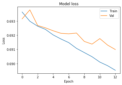
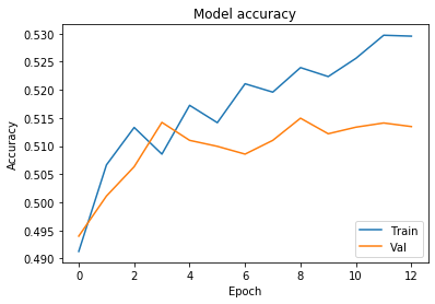
Train the Neural Network model and save trainig outputs ‘history’ variable
We will train the model 13 times and uploud batches with 500 items from our training dataset for one training iteration.
cell_timer = MeasureTime()
history = model.fit(X_train, Y_train,batch_size=500, epochs=13,validation_data=(X_val, Y_val))
cell_timer.kill()
Train on 18778 samples, validate on 9389 samples
Epoch 1/13
18778/18778 [==============================] - 7s 381us/step - loss: 0.6936 - acc: 0.4913 - val_loss: 0.6931 - val_acc: 0.4940
Epoch 2/13
18778/18778 [==============================] - 1s 50us/step - loss: 0.6930 - acc: 0.5067 - val_loss: 0.6938 - val_acc: 0.5011
Epoch 3/13
18778/18778 [==============================] - 1s 42us/step - loss: 0.6926 - acc: 0.5133 - val_loss: 0.6927 - val_acc: 0.5063
Epoch 4/13
18778/18778 [==============================] - 1s 50us/step - loss: 0.6924 - acc: 0.5086 - val_loss: 0.6925 - val_acc: 0.5142
Epoch 5/13
18778/18778 [==============================] - 1s 48us/step - loss: 0.6920 - acc: 0.5173 - val_loss: 0.6923 - val_acc: 0.5110
Epoch 6/13
18778/18778 [==============================] - 1s 49us/step - loss: 0.6917 - acc: 0.5142 - val_loss: 0.6921 - val_acc: 0.5100
Epoch 7/13
18778/18778 [==============================] - 1s 48us/step - loss: 0.6915 - acc: 0.5211 - val_loss: 0.6921 - val_acc: 0.5086
Epoch 8/13
18778/18778 [==============================] - 1s 51us/step - loss: 0.6911 - acc: 0.5196 - val_loss: 0.6921 - val_acc: 0.5110
Epoch 9/13
18778/18778 [==============================] - 1s 51us/step - loss: 0.6908 - acc: 0.5240 - val_loss: 0.6916 - val_acc: 0.5150
Epoch 10/13
18778/18778 [==============================] - ETA: 0s - loss: 0.6905 - acc: 0.522 - 1s 50us/step - loss: 0.6905 - acc: 0.5224 - val_loss: 0.6914 - val_acc: 0.5122
Epoch 11/13
18778/18778 [==============================] - 1s 48us/step - loss: 0.6901 - acc: 0.5256 - val_loss: 0.6918 - val_acc: 0.5134
Epoch 12/13
18778/18778 [==============================] - 1s 51us/step - loss: 0.6898 - acc: 0.5297 - val_loss: 0.6913 - val_acc: 0.5141
Epoch 13/13
18778/18778 [==============================] - 1s 46us/step - loss: 0.6895 - acc: 0.5296 - val_loss: 0.6910 - val_acc: 0.5135
Plot the charts to see model training loss and validation loss
# Chart 1 - Model Loss
#plt.subplot(331)
plt.plot(history.history['loss'])
plt.plot(history.history['val_loss'])
plt.title('Model loss')
plt.ylabel('Loss')
plt.xlabel('Epoch')
plt.legend(['Train', 'Val'], loc='upper right')
plt.show()


# Chart 2 - Model Accuracy
#plt.subplot(332)
plt.plot(history.history['acc'])
plt.plot(history.history['val_acc'])
plt.title('Model accuracy')
plt.ylabel('Accuracy')
plt.xlabel('Epoch')
plt.legend(['Train', 'Val'], loc='lower right')
plt.show()
1.5 - Test the model against new data
test_loss, test_acc = model.evaluate(X_test, Y_test)
print('Test accuracy:', test_acc)
9390/9390 [==============================] - 2s 219us/step
Test accuracy: 0.5175718849967209
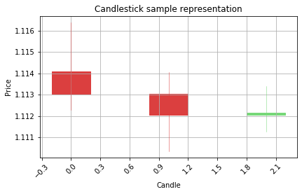
Visualize the predictions on the candlestick charts to see the patterns
Belowe there is a function to filter out the low confidence predictions from the model by using the alpha distance variable. If the prediction value is close to 0, that means the prediction is 0, the same case wth prediction 1, if the predicted value is closer to 1 instead of 0, it means the model predicted the value 1. If the prediction value is closer to its target, that means the confidence of the prediction is biger. Less distance to target prediction value, better the confidence. Please make sure that this approach works only with binary classification problems.
cell_timer = MeasureTime()
counter = 0
won = 0
lost = 0
test = model.predict(X_test)
alpha_distance = 0.35

for a in test:
    #print(a)
    if a > (1-alpha_distance) or a < alpha_distance :
        print(a)
        if Y_test[counter] == 1:print('Correct prediction is Bullish')
        if Y_test[counter] == 0:print('Correct prediction is Bearish')
        if a > (1-alpha_distance):print('Model prediction is Bullish')
        if a < alpha_distance:print('Model prediction is Bearish')

        if (a > (1-alpha_distance) and Y_test[counter] == 1) or (a < alpha_distance and Y_test[counter] == 0):
            won=won+1
            print('WON')
        else:
            print('LOST')
            lost=lost+1

        graph_data_ohlc(X_test_raw[counter])

    counter=counter+1
print('Won: ' + str(won) + ' Lost: ' + str(lost))
print('Success rate: ' + str(round((won*100)/(won+lost),2)) + '%')
cell_timer.kill()
[0.3420222]
Correct prediction is Bearish
Model prediction is Bearish
WON
[0.24589519]
Correct prediction is Bearish
Model prediction is Bearish
WON
[0.24589519]
Correct prediction is Bearish
Model prediction is Bearish
WON
[0.24589519]
Correct prediction is Bearish
Model prediction is Bearish
WON
[0.24589519]
Correct prediction is Bearish
Model prediction is Bearish
WON
[0.24589519]
Correct prediction is Bearish
Model prediction is Bearish
WON
[0.24589519]
Correct prediction is Bearish
Model prediction is Bearish
WON
[0.24589519]
Correct prediction is Bearish
Model prediction is Bearish
WON
[0.31519535]
Correct prediction is Bearish
Model prediction is Bearish
WON
[0.24589519]
Correct prediction is Bearish
Model prediction is Bearish
WON
Won: 52 Lost: 4
Success rate: 92.86%
Looks like we manage the get awesome results with our model after manipulating the alpha_distance value.
Won: 52 Lost: 4
Success rate: 92.86%
Test period: 13 Months
Thats huge!
1.6 - Check the model features importance
But the game is not over, when we have our model achieving awesome results on the test data, it is time to move in to data out of the sample (data that is not related to the previous data and the deep learning model never had contact with this kind of data) or to the live data. We will try both of those approaches.
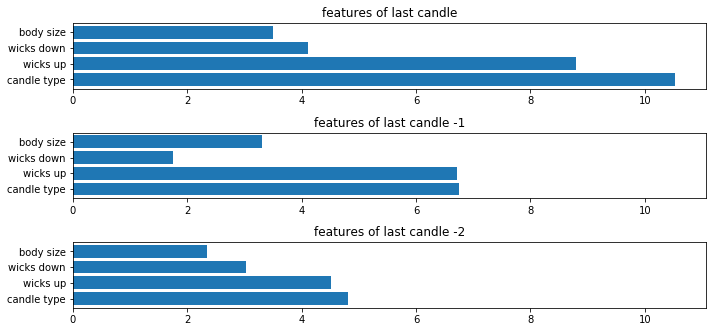
Before will will start making out of the sample test, let’s check which features were the most important for the model to make predictions.
def get_feature_importance(model,X_train_dataset,feature_names):
    pred_x = model.predict(X_train_dataset)

    random_ind = np.random.choice(X_train.shape[0], 1000, replace=False)

    data = X_train[random_ind[0:500]]
    e = shap.DeepExplainer((model.layers[0].input, model.layers[-1].output),data)
    test1 = X_train[random_ind[500:1000]]
    shap_val = e.shap_values(test1)
    shap_val = np.array(shap_val)
    shap_val = np.reshape(shap_val,(int(shap_val.shape[1]),int(shap_val.shape[2]),int(shap_val.shape[3])))
    shap_abs = np.absolute(shap_val)
    sum_0 = np.sum(shap_abs,axis=0)
    x_pos = [i for i, _ in enumerate(f_names)]

    plt.figure(figsize=(10,6))

    plt1 = plt.subplot(4,1,1)
    plt1.barh(x_pos,sum_0[2])
    plt1.set_yticks(x_pos)
    plt1.set_yticklabels(feature_names)
    plt1.set_title('features of last candle')

    plt2 = plt.subplot(4,1,2,sharex=plt1)
    plt2.barh(x_pos,sum_0[1])
    plt2.set_yticks(x_pos)
    plt2.set_yticklabels(feature_names)
    plt2.set_title('features of last candle -1')

    plt3 = plt.subplot(4,1,3,sharex=plt1)
    plt3.barh(x_pos,sum_0[0])
    plt3.set_yticks(x_pos)
    plt3.set_yticklabels(feature_names)
    plt3.set_title('features of last candle -2')

    plt.tight_layout()
    plt.show()
cell_timer = MeasureTime()
features_list=['candle type','wicks up', 'wicks down', 'body size']
get_feature_importance(model,X_train,features_list)
cell_timer.kill()
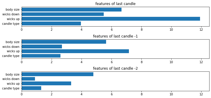
Now we can see that model trained itself in a way to pay the most attention to the first candle and the wicks up parameter. The last candle is also less important than the others when it comes to making prediction.
1.7 - The BIG DATA
Now it is time to download the big dataset of more than
0.7 Milion of historical 1 hour candlestciks from 7 currency pairs
We will download our historical dataset from ducascopy website in form of many CSV files. https://www.dukascopy.com/trading-tools/widgets/quotes/historical_data_feed
*EURUSD
*GBPUSD
*USDCAD
*NZDUSD
*USDJPY
*AUDUSD
*USDCHF All of the above datasets are for time period od 2003-2019
EURUSD
cell_timer = MeasureTime()
EURUSD_dataset = pd.read_csv('Hour/EURUSD.csv')
del EURUSD_dataset['Gmt time']
del EURUSD_dataset['Volume']
X,Y, X_raw = my_generator_candle_X_Y(EURUSD_dataset.values,3,MinMax=False)
cell_timer.kill()
GBPUSD
cell_timer = MeasureTime()
GBPUSD_dataset = pd.read_csv('Hour/GBPUSD.csv')
del GBPUSD_dataset['Gmt time']
del GBPUSD_dataset['Volume']
X2,Y2, X2_raw = my_generator_candle_X_Y(GBPUSD_dataset.values,3,MinMax=False)
cell_timer.kill()
USDCAD
cell_timer = MeasureTime()
USDCAD_dataset = pd.read_csv('Hour/USDCAD.csv')
del USDCAD_dataset['Gmt time']
del USDCAD_dataset['Volume']
X3,Y3, X3_raw = my_generator_candle_X_Y(USDCAD_dataset.values,3,MinMax=False)
cell_timer.kill()
NZDUSD
cell_timer = MeasureTime()
NZDUSD_dataset = pd.read_csv('Hour/NZDUSD.csv')
del NZDUSD_dataset['Gmt time']
del NZDUSD_dataset['Volume']
X4,Y4, X4_raw = my_generator_candle_X_Y(NZDUSD_dataset.values,3,MinMax=False)
cell_timer.kill()
USDJPY
cell_timer = MeasureTime()
USDJPY_dataset = pd.read_csv('Hour/USDJPY.csv')
del USDJPY_dataset['Gmt time']
del USDJPY_dataset['Volume']
X5,Y5, X5_raw = my_generator_candle_X_Y(USDJPY_dataset.values,3,MinMax=False)
cell_timer.kill()
AUDUSD
cell_timer = MeasureTime()
AUDUSD_dataset = pd.read_csv('Hour/AUDUSD.csv')
del AUDUSD_dataset['Gmt time']
del AUDUSD_dataset['Volume']
X6, Y6, X6_raw = my_generator_candle_X_Y(AUDUSD_dataset.values,3,MinMax=False)
cell_timer.kill()
Time elapsed: 00:03:30
USDCHF
cell_timer = MeasureTime()
USDCHF_dataset = pd.read_csv('Hour/USDCHF.csv')
del USDCHF_dataset['Gmt time']
del USDCHF_dataset['Volume']
X7,Y7, X7_raw = my_generator_candle_X_Y(USDCHF_dataset.values,3,MinMax=False)
cell_timer.kill()
Time elapsed: 00:03:35
Below function is the update function to calculate the potential accuracy of the model with alpha distance parameter
Aplha distance = maximum accetable distance from predicted value to prediction target.
For example if we want to predict 1 or 0 (1=Bullish , 0=Bearish) and our model will return 0.70, it means that distance to 1 is 0.3 and distance to 0 i 0.7. Smaller the distance = higher accuracy during the prediction
def evaluate_candle_model(model_passed,alpha_distance,X,Y,X_raw,print_charts=False):
    counter = 0
    won = 0
    lost = 0
    test = model_passed.predict(X)
    for a in test:
        if a > (1-alpha_distance) or a < alpha_distance :
            if print_charts==True:
                print(a)
                if Y[counter] == 1:print('Correct prediction is Bullish')
                if Y[counter] == 0:print('Correct prediction is Bearish')
                if a > (1-alpha_distance):print('Model prediction is Bullish')
                if a < alpha_distance:print('Model prediction is Bearish')
            if (a > (1-alpha_distance) and Y[counter] == 1) or (a < alpha_distance and Y[counter] == 0):
                won=won+1
                if print_charts==True:print('WON')
            else:
                if print_charts==True:print('LOST')
                lost=lost+1

            if print_charts==True:graph_data_ohlc(X_raw[counter])

        counter=counter+1
    if won != 0:
        print('Won: ' + str(won) + ' Lost: ' + str(lost))
        print('Success rate: ' + str(round((won*100)/(won+lost),2)) + '%')
    return [won+lost,won,lost]
Lets calculate how our trained model will perform on larger dataset that the model had no access to during the training.
cell_timer = MeasureTime()

alpha_distance = 0.30

total=0
win=0
loss=0

print('EURUSD Prediction:')
evaluation = evaluate_candle_model(model,alpha_distance,X,Y,X_raw,print_charts=False)
total = total + evaluation[0]
win = win + evaluation[1]
loss = loss + evaluation[2]
print('---------------------------------------------------')
print('GBPUSD Prediction:')
evaluation = evaluate_candle_model(model,alpha_distance,X2,Y2,X2_raw,print_charts=False)
total = total + evaluation[0]
win = win + evaluation[1]
loss = loss + evaluation[2]
print('---------------------------------------------------')
print('USDCAD Prediction:')
evaluation = evaluate_candle_model(model,alpha_distance,X3,Y3,X3_raw,print_charts=False)
total = total + evaluation[0]
win = win + evaluation[1]
loss = loss + evaluation[2]
print('---------------------------------------------------')
print('NZDUSD Prediction:')
evaluation = evaluate_candle_model(model,alpha_distance,X4,Y4,X4_raw,print_charts=False)
total = total + evaluation[0]
win = win + evaluation[1]
loss = loss + evaluation[2]
print('---------------------------------------------------')
print('USDJPY Prediction:')
evaluation = evaluate_candle_model(model,alpha_distance,X5,Y5,X5_raw,print_charts=False)
total = total + evaluation[0]
win = win + evaluation[1]
loss = loss + evaluation[2]
print('---------------------------------------------------')
print('AUDUSD Prediction:')
evaluation = evaluate_candle_model(model,alpha_distance,X6,Y6,X6_raw,print_charts=False)
total = total + evaluation[0]
win = win + evaluation[1]
loss = loss + evaluation[2]
print('---------------------------------------------------')
print('USDCHF Prediction:')
evaluation = evaluate_candle_model(model,alpha_distance,X7,Y7,X7_raw,print_charts=False)
total = total + evaluation[0]
win = win + evaluation[1]
loss = loss + evaluation[2]
print('---------------------------------------------------')
print('PREDICTIONS WIN: ' + str(win))
print('PREDICTIONS LOSS: ' + str(loss))
print('PREDICTIONS ACCURACY: ' + str(round((win*100)/(win+loss),2)) + '%')
print('PREDICTIONS PER MONTH: ' + str(round(total/192,0)))
print('PREDICTIONS TEST PERIOD: ' + '16 YEARS (2013-2019)')
cell_timer.kill()
EURUSD Prediction:
Won: 202 Lost: 18
Success rate: 91.82%
---------------------------------------------------
GBPUSD Prediction:
Won: 183 Lost: 11
Success rate: 94.33%
---------------------------------------------------
USDCAD Prediction:
Won: 201 Lost: 8
Success rate: 96.17%
---------------------------------------------------
NZDUSD Prediction:
Won: 225 Lost: 14
Success rate: 94.14%
---------------------------------------------------
US6DJPY Prediction:
Won: 187 Lost: 9
Success rate: 95.41%
---------------------------------------------------
AUDUSD Prediction:
Won: 700 Lost: 81
Success rate: 89.63%
---------------------------------------------------
USDCHF Prediction:
Won: 191 Lost: 11
Success rate: 94.55%
---------------------------------------------------
PREDICTIONS WIN: 1889
PREDICTIONS LOSS: 152
PREDICTIONS ACCURACY: 92.55%
PREDICTIONS PER MONTH: 11.0
PREDICTIONS TEST PERIOD: 16 YEARS (2013-2019)
Time elapsed: 00:06:55
The results are very promising, 92% on 16 year data period. But before we will move further, lets check how many Bullish and Bearish predictions we had.
cell_timer = MeasureTime()
EURUSD_pred_check = model.predict(X)
GBPUSD_pred_check = model.predict(X2)
USDCAD_pred_check = model.predict(X3)
NZDUSD_pred_check = model.predict(X4)
USDJPY_pred_check = model.predict(X5)
AUDUSD_pred_check = model.predict(X6)
USDCHF_pred_check = model.predict(X7)
cell_timer.kill()
Time elapsed: 00:01:44
cell_timer = MeasureTime()
all_currencies_predictions = np.concatenate([EURUSD_pred_check, GBPUSD_pred_check, USDCAD_pred_check,NZDUSD_pred_check,USDJPY_pred_check,AUDUSD_pred_check,USDCHF_pred_check], axis=0)
cell_timer.kill()
Time elapsed: 00:00:00
all_currencies_predictions.shape
(703419, 1)
cell_timer = MeasureTime()
alpha_distance_value = 0.3
bullish_count=0
bearish_count=0
for pred in all_currencies_predictions:
    if pred < alpha_distance_value: bearish_count=bearish_count+1
    if pred > (1-alpha_distance_value): bullish_count=bullish_count+1
print('Bullish predictions in total: ' + str(bullish_count))
print('Bearish predictions in total: ' + str(bearish_count))
print('Predictions in total: ' + str(bullish_count+bearish_count))
cell_timer.kill()
Bullish predictions in total: 0
Bearish predictions in total: 2041
Predictions in total: 2041
Time elapsed: 00:00:03
Looks like our model learned perfectly how to predict only the bearish candle. All of the predictions above alpha distance are for bearish candles. This is good however the goal is to make predictions with high accuracy for Bearish and Bullish candles. Let’s move further and investigate what could be the problem in here.
Anyway, the results might have something valuable in it, so for now on let’s just save the model in case for future reference.
model.save("predict_candlestick_1.7.h5")
print("Saved model to disk")
Saved model to disk
1.8 Multiple LSTM layers
Now we know how the model with low level of layers and unit/neurons perform on our data, but what if we extend the number of layeres and neurons. We will give to our model more room for training to remember the data. We will also give more data for training instead of a last time. We will take GBP/USD and EUR/USD during period 2003-2019 for training. Maybe increasing the dataset will solve our problem of model learning only to make predictions in one direction.
Get the training data:
cell_timer = MeasureTime()
merged_X = np.concatenate((X, X2), axis=0)
cell_timer.kill()
Time elapsed: 00:00:00
cell_timer = MeasureTime()
merged_Y = np.concatenate((Y, Y2), axis=0)
cell_timer.kill()
Time elapsed: 00:00:00
cell_timer = MeasureTime()
merged_X_rwa = np.concatenate((X_raw, X2_raw), axis=0)
cell_timer.kill()
Time elapsed: 00:00:00
merged_X.shape
(202314, 3, 4)
merged_Y.shape
(202314,)
cell_timer = MeasureTime()
X_train_merged, X_val_and_test, Y_train_merged, Y_val_and_test = train_test_split(merged_X, merged_Y, test_size=0.5)
X_val_merged, X_test_merged, Y_val_merged, Y_test_merged = train_test_split(X_val_and_test, Y_val_and_test, test_size=0.5)

X_train_raw_merged, X_val_and_test_raw= train_test_split(merged_X_rwa, test_size=0.5)
X_val_raw_merged, X_test_raw_merged = train_test_split(X_val_and_test_raw, test_size=0.5)
cell_timer.kill()
Time elapsed: 00:00:00
The new model will be build from 6x LSTM layers with 12,24,24,24,12,6 neurons. You may also spot that right now we have also added layers called “Dropout”
Droput is basically a layer that each time data is passing through it, the layer drops some percentage of this data to avoid overfitting problem.
In simple worlds, it will allow our model to learn longer without overfitting.
from keras import layers
from keras.optimizers import RMSprop

model = Sequential()

model.add(layers.CuDNNLSTM(units = 12,return_sequences=True, input_shape = (None, X.shape[-1])))
model.add(Dropout(0.3))
model.add(layers.CuDNNLSTM(units = 24,return_sequences=True,))
model.add(Dropout(0.3))
model.add(layers.CuDNNLSTM(units = 24,return_sequences=True))
model.add(Dropout(0.3))
model.add(layers.CuDNNLSTM(units = 24,return_sequences=True))
model.add(Dropout(0.2))
model.add(layers.CuDNNLSTM(units = 12,return_sequences=True))
model.add(Dropout(0.2))
model.add(layers.CuDNNLSTM(units = 6))

model.add(layers.Dense(units = 1,activation='sigmoid'))

model.compile(optimizer='rmsprop', loss='binary_crossentropy', metrics=['acc'])
model.summary()
Model: "sequential_3"
_________________________________________________________________
Layer (type)                 Output Shape              Param #
=================================================================
cu_dnnlstm_9 (CuDNNLSTM)     (None, None, 12)          864
_________________________________________________________________
dropout_6 (Dropout)          (None, None, 12)          0
_________________________________________________________________
cu_dnnlstm_10 (CuDNNLSTM)    (None, None, 24)          3648
_________________________________________________________________
dropout_7 (Dropout)          (None, None, 24)          0
_________________________________________________________________
cu_dnnlstm_11 (CuDNNLSTM)    (None, None, 24)          4800
_________________________________________________________________
dropout_8 (Dropout)          (None, None, 24)          0
_________________________________________________________________
cu_dnnlstm_12 (CuDNNLSTM)    (None, None, 24)          4800
_________________________________________________________________
dropout_9 (Dropout)          (None, None, 24)          0
_________________________________________________________________
cu_dnnlstm_13 (CuDNNLSTM)    (None, None, 12)          1824
_________________________________________________________________
dropout_10 (Dropout)         (None, None, 12)          0
_________________________________________________________________
cu_dnnlstm_14 (CuDNNLSTM)    (None, 6)                 480
_________________________________________________________________
dense_3 (Dense)              (None, 1)                 7
=================================================================
Total params: 16,423
Trainable params: 16,423
Non-trainable params: 0
_________________________________________________________________
Training process:
cell_timer = MeasureTime()
history = model.fit(X_train_merged, Y_train_merged,batch_size=500, epochs=50,validation_data=(X_val_merged, Y_val_merged))
cell_timer.kill()
Train on 101157 samples, validate on 50578 samples
Epoch 1/50
101157/101157 [==============================] - 13s 129us/step - loss: 0.6932 - acc: 0.4999 - val_loss: 0.6932 - val_acc: 0.4956
Epoch 2/50
101157/101157 [==============================] - 11s 106us/step - loss: 0.6932 - acc: 0.4998 - val_loss: 0.6932 - val_acc: 0.4995
Epoch 3/50
101157/101157 [==============================] - 11s 107us/step - loss: 0.6932 - acc: 0.4995 - val_loss: 0.6931 - val_acc: 0.5044
Epoch 4/50
101157/101157 [==============================] - 11s 106us/step - loss: 0.6932 - acc: 0.4999 - val_loss: 0.6931 - val_acc: 0.5025
Epoch 5/50
101157/101157 [==============================] - 11s 108us/step - loss: 0.6932 - acc: 0.4997 - val_loss: 0.6932 - val_acc: 0.5009
Epoch 6/50
101157/101157 [==============================] - 11s 107us/step - loss: 0.6931 - acc: 0.5047 - val_loss: 0.6932 - val_acc: 0.5026
Epoch 7/50
101157/101157 [==============================] - 11s 107us/step - loss: 0.6931 - acc: 0.5043 - val_loss: 0.6931 - val_acc: 0.5017
Epoch 8/50
101157/101157 [==============================] - 11s 107us/step - loss: 0.6928 - acc: 0.5072 - val_loss: 0.6931 - val_acc: 0.5049
Epoch 9/50
101157/101157 [==============================] - 11s 108us/step - loss: 0.6925 - acc: 0.5069 - val_loss: 0.6923 - val_acc: 0.5059
Epoch 10/50
101157/101157 [==============================] - 11s 108us/step - loss: 0.6922 - acc: 0.5074 - val_loss: 0.6923 - val_acc: 0.5043
Epoch 11/50
101157/101157 [==============================] - 10s 102us/step - loss: 0.6921 - acc: 0.5095 - val_loss: 0.6920 - val_acc: 0.5100
Epoch 12/50
101157/101157 [==============================] - 11s 106us/step - loss: 0.6919 - acc: 0.5093 - val_loss: 0.6922 - val_acc: 0.5096
Epoch 13/50
101157/101157 [==============================] - 11s 107us/step - loss: 0.6919 - acc: 0.5117 - val_loss: 0.6919 - val_acc: 0.5123
Epoch 14/50
101157/101157 [==============================] - 11s 107us/step - loss: 0.6917 - acc: 0.5143 - val_loss: 0.6918 - val_acc: 0.5127
Epoch 15/50
101157/101157 [==============================] - 11s 108us/step - loss: 0.6916 - acc: 0.5157 - val_loss: 0.6917 - val_acc: 0.5129
Epoch 16/50
101157/101157 [==============================] - 11s 111us/step - loss: 0.6914 - acc: 0.5194 - val_loss: 0.6917 - val_acc: 0.5131
Epoch 17/50
101157/101157 [==============================] - 11s 107us/step - loss: 0.6913 - acc: 0.5180 - val_loss: 0.6913 - val_acc: 0.5200
Epoch 18/50
101157/101157 [==============================] - 11s 108us/step - loss: 0.6913 - acc: 0.5188 - val_loss: 0.6915 - val_acc: 0.5172
Epoch 19/50
101157/101157 [==============================] - 11s 108us/step - loss: 0.6911 - acc: 0.5205 - val_loss: 0.6915 - val_acc: 0.5154
Epoch 20/50
101157/101157 [==============================] - 11s 106us/step - loss: 0.6909 - acc: 0.5209 - val_loss: 0.6911 - val_acc: 0.5206
Epoch 21/50
101157/101157 [==============================] - 11s 106us/step - loss: 0.6910 - acc: 0.5197 - val_loss: 0.6911 - val_acc: 0.5226
Epoch 22/50
101157/101157 [==============================] - 11s 106us/step - loss: 0.6907 - acc: 0.5244 - val_loss: 0.6907 - val_acc: 0.5251
Epoch 23/50
101157/101157 [==============================] - 11s 106us/step - loss: 0.6907 - acc: 0.5239 - val_loss: 0.6907 - val_acc: 0.5248
Epoch 24/50
101157/101157 [==============================] - 11s 107us/step - loss: 0.6905 - acc: 0.5239 - val_loss: 0.6909 - val_acc: 0.5245
Epoch 25/50
101157/101157 [==============================] - 11s 108us/step - loss: 0.6908 - acc: 0.5222 - val_loss: 0.6905 - val_acc: 0.5258
Epoch 26/50
101157/101157 [==============================] - 11s 109us/step - loss: 0.6905 - acc: 0.5245 - val_loss: 0.6904 - val_acc: 0.5269
Epoch 27/50
101157/101157 [==============================] - 11s 106us/step - loss: 0.6906 - acc: 0.5240 - val_loss: 0.6904 - val_acc: 0.5253
Epoch 28/50
101157/101157 [==============================] - 11s 109us/step - loss: 0.6903 - acc: 0.5271 - val_loss: 0.6906 - val_acc: 0.5244
Epoch 29/50
101157/101157 [==============================] - 11s 108us/step - loss: 0.6903 - acc: 0.5266 - val_loss: 0.6904 - val_acc: 0.5253
Epoch 30/50
101157/101157 [==============================] - 11s 110us/step - loss: 0.6903 - acc: 0.5269 - val_loss: 0.6901 - val_acc: 0.5274
Epoch 31/50
101157/101157 [==============================] - 11s 110us/step - loss: 0.6901 - acc: 0.5284 - val_loss: 0.6902 - val_acc: 0.5277
Epoch 32/50
101157/101157 [==============================] - 11s 106us/step - loss: 0.6899 - acc: 0.5288 - val_loss: 0.6902 - val_acc: 0.5277
Epoch 33/50
101157/101157 [==============================] - 11s 106us/step - loss: 0.6900 - acc: 0.5276 - val_loss: 0.6902 - val_acc: 0.5276
Epoch 34/50
101157/101157 [==============================] - 11s 109us/step - loss: 0.6899 - acc: 0.5280 - val_loss: 0.6901 - val_acc: 0.5279
Epoch 35/50
101157/101157 [==============================] - 11s 109us/step - loss: 0.6901 - acc: 0.5278 - val_loss: 0.6901 - val_acc: 0.5285
Epoch 36/50
101157/101157 [==============================] - 11s 110us/step - loss: 0.6901 - acc: 0.5287 - val_loss: 0.6902 - val_acc: 0.5294
Epoch 37/50
101157/101157 [==============================] - 11s 108us/step - loss: 0.6897 - acc: 0.5291 - val_loss: 0.6904 - val_acc: 0.5272
Epoch 38/50
101157/101157 [==============================] - 11s 107us/step - loss: 0.6900 - acc: 0.5286 - val_loss: 0.6901 - val_acc: 0.5275
Epoch 39/50
101157/101157 [==============================] - 11s 108us/step - loss: 0.6898 - acc: 0.5298 - val_loss: 0.6905 - val_acc: 0.5254
Epoch 40/50
101157/101157 [==============================] - 11s 109us/step - loss: 0.6900 - acc: 0.5277 - val_loss: 0.6904 - val_acc: 0.5283
Epoch 41/50
101157/101157 [==============================] - 11s 107us/step - loss: 0.6900 - acc: 0.5297 - val_loss: 0.6901 - val_acc: 0.5285
Epoch 42/50
101157/101157 [==============================] - 11s 106us/step - loss: 0.6900 - acc: 0.5302 - val_loss: 0.6902 - val_acc: 0.5281
Epoch 43/50
101157/101157 [==============================] - 11s 109us/step - loss: 0.6897 - acc: 0.5301 - val_loss: 0.6904 - val_acc: 0.5266
Epoch 44/50
101157/101157 [==============================] - 11s 109us/step - loss: 0.6898 - acc: 0.5292 - val_loss: 0.6900 - val_acc: 0.5264
Epoch 45/50
101157/101157 [==============================] - 11s 108us/step - loss: 0.6899 - acc: 0.5285 - val_loss: 0.6903 - val_acc: 0.5289
Epoch 46/50
101157/101157 [==============================] - 11s 110us/step - loss: 0.6896 - acc: 0.5296 - val_loss: 0.6904 - val_acc: 0.5280
Epoch 47/50
101157/101157 [==============================] - 11s 109us/step - loss: 0.6896 - acc: 0.5309 - val_loss: 0.6901 - val_acc: 0.5282
Epoch 48/50
101157/101157 [==============================] - 11s 110us/step - loss: 0.6897 - acc: 0.5291 - val_loss: 0.6901 - val_acc: 0.5295
Epoch 49/50
101157/101157 [==============================] - 11s 106us/step - loss: 0.6895 - acc: 0.5301 - val_loss: 0.6902 - val_acc: 0.5294
Epoch 50/50
101157/101157 [==============================] - 11s 109us/step - loss: 0.6897 - acc: 0.5298 - val_loss: 0.6900 - val_acc: 0.5293
Time elapsed: 00:09:09
# Chart 1 - Model Loss
#plt.subplot(331)
plt.plot(history.history['loss'])
plt.plot(history.history['val_loss'])
plt.title('Model loss')
plt.ylabel('Loss')
plt.xlabel('Epoch')
plt.legend(['Train', 'Val'], loc='upper right')
plt.show()


# Chart 2 - Model Accuracy
#plt.subplot(332)
plt.plot(history.history['acc'])
plt.plot(history.history['val_acc'])
plt.title('Model accuracy')
plt.ylabel('Accuracy')
plt.xlabel('Epoch')
plt.legend(['Train', 'Val'], loc='lower right')
plt.show()
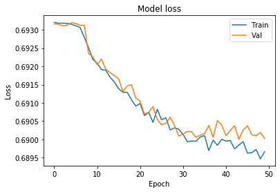
Looks like our model is getting overfitted by the ~25th epoch. let’s train it again only for 25 epochs.
from keras import layers
from keras.optimizers import RMSprop

model = Sequential()

model.add(layers.CuDNNLSTM(units = 12,return_sequences=True, input_shape = (None, X.shape[-1])))
model.add(Dropout(0.3))
model.add(layers.CuDNNLSTM(units = 24,return_sequences=True,))
model.add(Dropout(0.3))
model.add(layers.CuDNNLSTM(units = 24,return_sequences=True))
model.add(Dropout(0.3))
model.add(layers.CuDNNLSTM(units = 24,return_sequences=True))
model.add(Dropout(0.2))
model.add(layers.CuDNNLSTM(units = 12,return_sequences=True))
model.add(Dropout(0.2))
model.add(layers.CuDNNLSTM(units = 6))

model.add(layers.Dense(units = 1,activation='sigmoid'))

model.compile(optimizer='rmsprop', loss='binary_crossentropy', metrics=['acc'])
cell_timer = MeasureTime()
history = model.fit(X_train_merged, Y_train_merged,batch_size=500, epochs=25,validation_data=(X_val_merged, Y_val_merged))
cell_timer.kill()
Train on 101157 samples, validate on 50578 samples
Epoch 1/25
101157/101157 [==============================] - 14s 135us/step - loss: 0.6932 - acc: 0.4987 - val_loss: 0.6932 - val_acc: 0.4956
Epoch 2/25
101157/101157 [==============================] - 11s 108us/step - loss: 0.6932 - acc: 0.4978 - val_loss: 0.6931 - val_acc: 0.4994
Epoch 3/25
101157/101157 [==============================] - 11s 109us/step - loss: 0.6932 - acc: 0.5005 - val_loss: 0.6931 - val_acc: 0.5044
Epoch 4/25
101157/101157 [==============================] - 11s 109us/step - loss: 0.6931 - acc: 0.5017 - val_loss: 0.6931 - val_acc: 0.5059
Epoch 5/25
101157/101157 [==============================] - 11s 108us/step - loss: 0.6931 - acc: 0.5035 - val_loss: 0.6933 - val_acc: 0.5010
Epoch 6/25
101157/101157 [==============================] - 11s 107us/step - loss: 0.6930 - acc: 0.5039 - val_loss: 0.6931 - val_acc: 0.5026
Epoch 7/25
101157/101157 [==============================] - 11s 106us/step - loss: 0.6930 - acc: 0.5069 - val_loss: 0.6931 - val_acc: 0.5034
Epoch 8/25
101157/101157 [==============================] - 11s 110us/step - loss: 0.6929 - acc: 0.5082 - val_loss: 0.6930 - val_acc: 0.5015
Epoch 9/25
101157/101157 [==============================] - 11s 107us/step - loss: 0.6926 - acc: 0.5090 - val_loss: 0.6928 - val_acc: 0.5047
Epoch 10/25
101157/101157 [==============================] - 11s 109us/step - loss: 0.6923 - acc: 0.5099 - val_loss: 0.6925 - val_acc: 0.5030
Epoch 11/25
101157/101157 [==============================] - 11s 111us/step - loss: 0.6921 - acc: 0.5122 - val_loss: 0.6924 - val_acc: 0.5110
Epoch 12/25
101157/101157 [==============================] - 11s 107us/step - loss: 0.6919 - acc: 0.5144 - val_loss: 0.6919 - val_acc: 0.5129
Epoch 13/25
101157/101157 [==============================] - 11s 107us/step - loss: 0.6917 - acc: 0.5164 - val_loss: 0.6925 - val_acc: 0.5048
Epoch 14/25
101157/101157 [==============================] - 11s 107us/step - loss: 0.6915 - acc: 0.5182 - val_loss: 0.6917 - val_acc: 0.5144
Epoch 15/25
101157/101157 [==============================] - 11s 106us/step - loss: 0.6914 - acc: 0.5200 - val_loss: 0.6914 - val_acc: 0.5162
Epoch 16/25
101157/101157 [==============================] - 11s 107us/step - loss: 0.6912 - acc: 0.5208 - val_loss: 0.6911 - val_acc: 0.5202
Epoch 17/25
101157/101157 [==============================] - 11s 109us/step - loss: 0.6910 - acc: 0.5217 - val_loss: 0.6911 - val_acc: 0.5219
Epoch 18/25
101157/101157 [==============================] - 11s 110us/step - loss: 0.6910 - acc: 0.5226 - val_loss: 0.6917 - val_acc: 0.5151
Epoch 19/25
101157/101157 [==============================] - 11s 109us/step - loss: 0.6908 - acc: 0.5262 - val_loss: 0.6908 - val_acc: 0.5236
Epoch 20/25
101157/101157 [==============================] - 11s 106us/step - loss: 0.6905 - acc: 0.5263 - val_loss: 0.6907 - val_acc: 0.5262
Epoch 21/25
101157/101157 [==============================] - 11s 107us/step - loss: 0.6905 - acc: 0.5271 - val_loss: 0.6906 - val_acc: 0.5262
Epoch 22/25
101157/101157 [==============================] - 11s 110us/step - loss: 0.6905 - acc: 0.5256 - val_loss: 0.6905 - val_acc: 0.5256
Epoch 23/25
101157/101157 [==============================] - 11s 104us/step - loss: 0.6905 - acc: 0.5263 - val_loss: 0.6905 - val_acc: 0.5262
Epoch 24/25
101157/101157 [==============================] - 11s 107us/step - loss: 0.6903 - acc: 0.5274 - val_loss: 0.6903 - val_acc: 0.5276
Epoch 25/25
101157/101157 [==============================] - 11s 108us/step - loss: 0.6902 - acc: 0.5278 - val_loss: 0.6906 - val_acc: 0.5272
Time elapsed: 00:04:37
# Chart 1 - Model Loss
#plt.subplot(331)
plt.plot(history.history['loss'])
plt.plot(history.history['val_loss'])
plt.title('Model loss')
plt.ylabel('Loss')
plt.xlabel('Epoch')
plt.legend(['Train', 'Val'], loc='upper right')
plt.show()


# Chart 2 - Model Accuracy
#plt.subplot(332)
plt.plot(history.history['acc'])
plt.plot(history.history['val_acc'])
plt.title('Model accuracy')
plt.ylabel('Accuracy')
plt.xlabel('Epoch')
plt.legend(['Train', 'Val'], loc='lower right')
plt.show()
Evaluate how good is the new model:
Concatonate all the curencies we got left and evaluate model on them
cell_timer = MeasureTime()
merged_curr_test_X = np.concatenate([X3,X4,X5,X6,X7], axis=0)
merged_curr_test_Y = np.concatenate([Y3,Y4,Y5,Y6,Y7], axis=0)
merged_curr_test_X_raw = np.concatenate([X3_raw,X4_raw,X5_raw,X6_raw,X7_raw], axis=0)
cell_timer.kill()
Time elapsed: 00:03:07
print(merged_curr_test_X.shape)
print(merged_curr_test_Y.shape)
print(merged_curr_test_X_raw.shape)
(501105, 3, 4)
(501105,)
(501105, 3, 4)
Evaluate:
cell_timer = MeasureTime()
merged_evaluation = evaluate_candle_model(model,0.3,merged_curr_test_X,merged_curr_test_Y,merged_curr_test_X_raw,print_charts=False)
cell_timer.kill()
Won: 1963 Lost: 397
Success rate: 83.18%
Check how many bullish and bearish trades we have:
cell_timer = MeasureTime()
all_currencies_predictions_merged = model.predict(merged_curr_test_X)
alpha_distance_value = 0.3
bullish_count=0
bearish_count=0
for pred in all_currencies_predictions_merged:
    if pred < alpha_distance_value: bearish_count=bearish_count+1
    if pred > (1-alpha_distance_value): bullish_count=bullish_count+1
print('Bullish predictions in total: ' + str(bullish_count))
print('Bearish predictions in total: ' + str(bearish_count))
print('Predictions in total: ' + str(bullish_count+bearish_count))
cell_timer.kill()
Bullish predictions in total: 0
Bearish predictions in total: 2360
Predictions in total: 2360
Time elapsed: 00:01:56
How those predictions are located over time?
def predictions_group(Predictions,timeperiod,alpha_distance_value):
    output = []
    templist=[]
    addval=0
    counter=0
    for pre in Predictions:
        if counter % timeperiod == 0:
            output.append(sum(templist.copy()))
            templist=[]
        if pre < alpha_distance_value: addval = 1
        elif pre > (1-alpha_distance_value): addval = 1
        else:
            addval = 0
        templist.append(addval)
        counter=counter+1
    return output
cell_timer = MeasureTime()
USDCAD_pred_month = predictions_group(model.predict(X3),2500,0.3)
NZDUSD_pred_month = predictions_group(model.predict(X4),2500,0.3)
USDJPY_pred_month = predictions_group(model.predict(X5),2500,0.3)
AUDUSD_pred_month = predictions_group(model.predict(X6),2500,0.3)
USDCHF_pred_month = predictions_group(model.predict(X7),2500,0.3)
cell_timer.kill()
Time elapsed: 00:00:56
import seaborn as sns
heat_map_data = np.random.random((5, 40))
a[0] = np.array(USDCAD_pred_month)
a[1] = np.array(NZDUSD_pred_month)
a[2] = np.array(USDJPY_pred_month[:40])
a[3] = np.array(AUDUSD_pred_month)
a[4] = np.array(USDCHF_pred_month[:40])
plt.figure(figsize=(20,10))
ax = sns.heatmap(a, linewidth=0.5)
#plt.imshow(a, cmap='hot', interpolation='nearest')
plt.title('Predictions per month')
plt.show()
We can see that our model is making predictions onlu in ~10 months out of 40 so it is 25%. It is not good.
Chek which feature is the most important
cell_timer = MeasureTime()
features_list_merged=['candle type','wicks up', 'wicks down', 'body size']
get_feature_importance(model,X_train_merged,features_list_merged)
cell_timer.kill()
Time elapsed: 00:00:30
Save the model for future reference
model.save("predict_candlestick_1.8.h5")
print("Saved model to disk")
Saved model to disk
1.9 - Conclusion
We did:
- loaded data from ducascopy servers
- format the data to time series
- format the OHLC data to candlestick data
- trained 2 LSTM models with diffrent parameters but both we accuracy above 80% in total
Problems:
- the model is learning only to predict bearish positions somehow, regardless diversified dataset.
- the model is overfitted, it is making predictions only in 10 months out of 40